Scale as a Coordinate

What the Cantor set looks like from inside a logarithm

Scale as a Coordinate

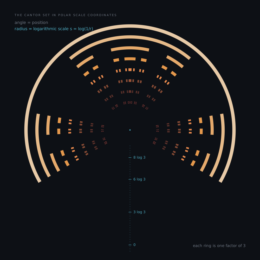
Everyone learns that the middle-thirds Cantor set has dimension $\log 2/\log 3$, and almost everyone moves on. But look at that number for a moment longer than usual. It is not a length, or an area, or a count. It is a ratio of two logarithms — which is to say, a slope. Something has been differentiated and nobody said what with respect to what.

This post takes that seriously. The claim is small but, I think, worth making carefully: if you stop treating "logarithmic scale" as a plotting convenience and start treating it as a coordinate, the self-similarity of the Cantor set stops being a verbal description and becomes a piece of visible geometry. And then, if you keep pushing, you arrive at the place where the mathematics is genuinely deep — which turns out not to be where the pretty reframing suggests.

1. The construction keeps two sets of books

The Cantor set $C$ is the attractor of two contractions,

$$f_0(x) = \tfrac{x}{3}, \qquad f_1(x) = \tfrac{x}{3} + \tfrac{2}{3},$$

and the standard picture of its construction is a stack of thinning bars. What that picture hides is that two entirely different quantities are being tracked down the page.

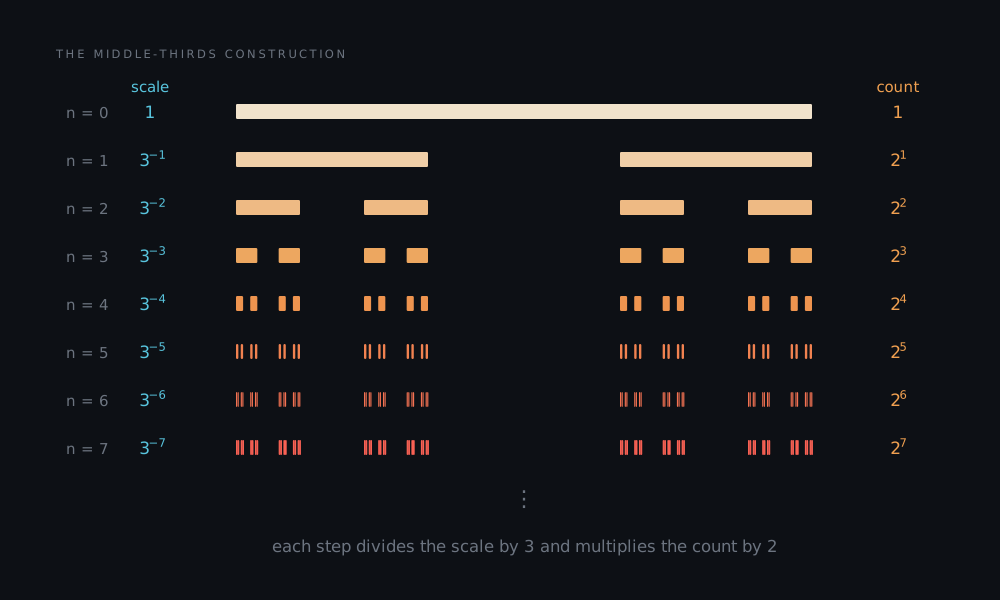
On the left, a scale: at level $n$ the surviving intervals have length $3^{-n}$. On the right, a count: there are $2^n$ of them. Both are geometric sequences, with different ratios, indexed by the same $n$. Everything interesting about $C$ is the relationship between those two columns, and the reason $\log 2/\log 3$ appears at all is that a ratio of geometric sequences is the only invariant they have.

2. Change the ruler

For $x, y > 0$, set

$$d_{\log}(x,y) = |\log x - \log y| = \left|\log \tfrac{x}{y}\right|.$$

This is a genuine metric on $(0,\infty)$ — in fact it makes $(0,\infty)$ isometric to $\mathbb{R}$ — and under it, equal ratios are equal distances. The points $1, 2, 4, 8, 16$, which crowd together at the left end of an ordinary ruler, become evenly spaced.

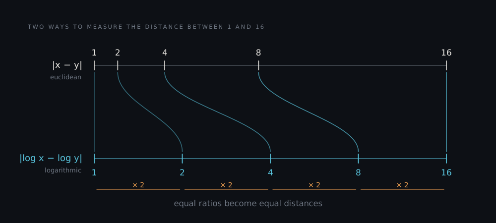
One honest caveat before going further, because it is easy to slide past it. We are not re-metrizing the Cantor set. $d_{\log}$ is not a metric on $C$; it is a metric on the space of resolutions at which we look at $C$. That is a different space, and the whole point of what follows is that it deserves to be treated as one. The move is not "replace $|x-y|$"; the move is "add an axis".

3. In the new ruler, the hierarchy is a lattice

Write $s = \log(1/r)$ for the logarithmic scale at resolution $r$. The Cantor construction's resolutions $r_n = 3^{-n}$ become

$$s_n = n \log 3,$$

an arithmetic progression: an evenly spaced lattice with spacing $\log 3$.

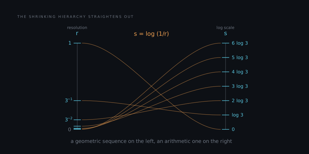
An infinite hierarchy that piles up at zero has been unrolled into something you can put a ruler against. Meanwhile the counts $N_n = 2^n$ become $\log N_n = n \log 2$, also arithmetic, with spacing $\log 2$. Two arithmetic progressions in the same index. Plot one against the other and the index disappears.

4. The dimension is an angle

$$\big(s_n,\ \Phi_n\big) = \big(n\log 3,\ n \log 2\big), \qquad n = 0, 1, 2, \dots$$

These points lie on a straight line through the origin. Draw the two axes with the same unit — and this matters, it is the whole trick — and the dimension becomes the tangent of an actual angle:

$$\tan\theta = \frac{\log 2}{\log 3} = d \approx 0.6309, \qquad \theta \approx 32.24^\circ.$$

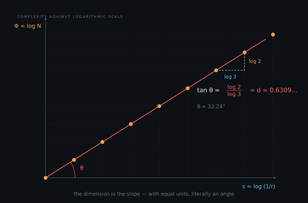
This is, I want to be clear, nothing more than the definition of box-counting dimension drawn carefully:

$$d = \lim_{r\to 0} \frac{\log N(r)}{\log(1/r)}.$$

No new mathematics has happened. But the picture has changed, and it changes what questions look natural. A slope invites you to ask about the second derivative. A line invites you to ask what happens when the data is not on it. Neither question is invited by the sentence "the Cantor set has dimension $\log 2/\log 3$."

5. The count is a staircase, not a line

Here is the first thing the picture makes obvious that the formula does not. $N(r)$ is only equal to $2^n$ at the special resolutions $r = 3^{-n}$. In between it is a step function, and $\Phi(s) = \log N(e^{-s})$ is a staircase that touches the line at the lattice scales and bulges above it everywhere else.

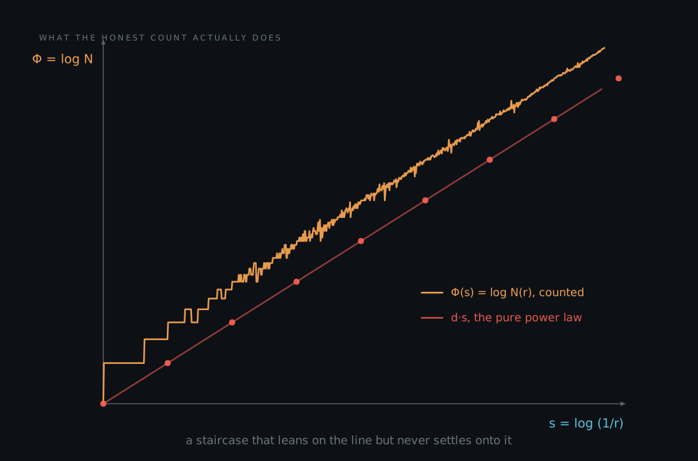
Write

$$\Phi(s) = d\,s + f(s).$$

The dimension is the part of $\Phi$ that survives being divided by $s$ as $s \to \infty$. Everything else — the entire function $f$ — is what the dimension throws away.

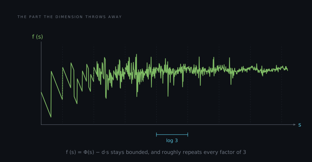
6. Where the oscillation becomes a theorem

Take the $\varepsilon$-neighbourhood of $C$ instead of a box count. The gaps of the Cantor set have length $3^{-n}$ with multiplicity $2^{n-1}$, and an $\varepsilon$-neighbourhood fills a gap of length $\ell$ to depth $\min(\ell, 2\varepsilon)$. Summing gives an exact elementary formula: with $m = \lfloor \log_3 \tfrac{1}{2\varepsilon} \rfloor$,

$$V(\varepsilon) = 2\varepsilon\,(2^m - 1) + \left(\tfrac{2}{3}\right)^{m}.$$

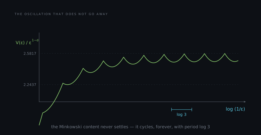
It does not converge. It settles into a waveform of amplitude about $4.6\%$ that repeats exactly, with period $\log 3$, forever. The Cantor set therefore has no Minkowski content: the limit that would define it simply does not exist.

This is not a numerical artefact and not a plotting choice — it is the substance. For self-similar subsets of the line satisfying the open set condition, Minkowski measurability is equivalent to the contraction ratios being non-lattice, i.e. to their logarithms not all being integer multiples of a common number. The middle-thirds set is maximally lattice: every ratio is $1/3$. The characterisation is due to Lapidus and Pomerance and, independently, to Falconer.^[1]

7. Objects with no single dimension

The reframing earns its keep when the data is not on a line. Take a Cantor-like set whose contraction ratio is $1/3$ for the first several levels and $1/9$ thereafter. It is a perfectly good compact set; it simply has no exponent.

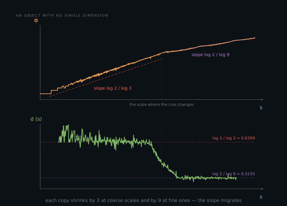
$\Phi$ has a bend in it, and the local slope

$$d(s) = \Phi'(s)$$ migrates from $\log 2/\log 3 \approx 0.631$ at coarse scales to $\log 2/\log 9 \approx 0.315$ at fine ones. (In the lower panel I measure the slope with a centred difference over exactly one period of the scaling, $s \pm \log 3$, which annihilates the log-periodic wobble instead of averaging it down; both scaling regimes here have periods commensurate with $\log 3$, which is the only reason that works.)

A single number cannot describe this object, but a function on the scale axis can. And once $d(s)$ is a function, the rest of the differential-geometric vocabulary shows up uninvited: $\Phi''$, the curvature of the scaling law; the amplitude and phase of the oscillation in $f$; the possibility that different parts of the set have different local $d(s)$, which is multifractality.

8. Where the oscillation actually lives

The last step is the one that convinced me the picture is pointing somewhere real. Encode the gaps as a Dirichlet series — the geometric zeta function of the Cantor string:

$$\zeta_C(s) = \sum_{n \ge 1} 2^{n-1} 3^{-ns} = \frac{3^{-s}}{1 - 2\cdot 3^{-s}}.$$

Its poles are exactly where $3^{s} = 2$, that is at

$$s = \frac{\log 2}{\log 3} + \frac{2\pi i k}{\log 3}, \qquad k \in \mathbb{Z}.$$

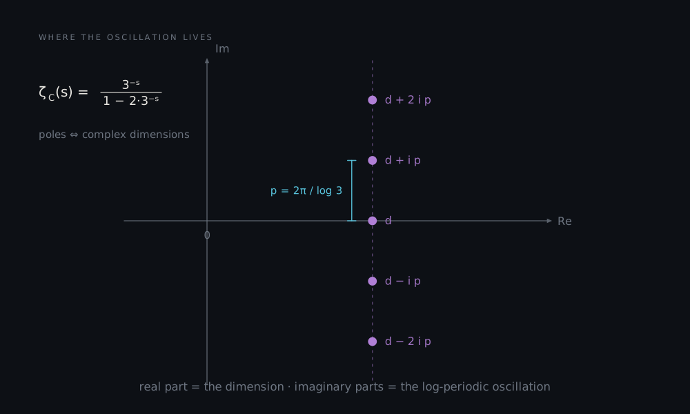
A vertical arithmetic lattice in the complex plane. The real part is the dimension. The imaginary parts are the oscillation — spacing $p = 2\pi/\log 3 \approx 5.72$, which is precisely the frequency conjugate to the period $\log 3$ we saw in the tube volume. The oscillation in §6 was not noise decorating the power law; it was the rest of the pole structure making itself visible.

Arriving somewhere already inhabited

I should confess how this post ends, because it is not how I expected it to end.

Drawing the Cantor set in scale coordinates feels like a discovery. The hierarchy of intervals settles into a lattice, the dimension turns into an angle, and it is tempting to believe you have stumbled onto a new way of seeing. So I did what one should always do with that feeling: I went looking for who had been here before me.

The first four sections, it turns out, are simply the definition of box dimension, drawn with care. That is not nothing. I would happily put these pictures in front of a lecture hall, because they make the definition visible. But a clearer picture of a known idea is a way of teaching, not a result.

The oscillations of the later sections had been found too, and thoroughly. Physicists know them as discrete scale invariance and log-periodic corrections to scaling, and they have chased them through rupture, earthquakes, diffusion-limited aggregation and financial time series; Sornette's review is where that trail begins.^[2] On the mathematical side, everything I was groping towards (fractal strings, geometric zeta functions, complex dimensions, tube formulas) already has a name and a home: the theory of complex dimensions built by Lapidus and van Frankenhuijsen. It is a mature theory, with monographs, not a gap waiting to be filled.^[3]

So the road I thought I was cutting through the forest was already paved. "Geometry of scale", in one dimension, is not an open frontier; it is largely another name for the theory of complex dimensions. If you ever feel the urge to build a framework here, read that literature first, and expect to meet your idea in it.

And yet, standing at the edge of the paved road, a few paths still lead off into the trees. They are narrower and less glamorous than the one I set out on, but I think they are genuinely unexplored.

The first leads away from perfect symmetry. The theory is at its sharpest for self-similar and self-conformal sets, objects that repeat themselves exactly. But most of what we measure in the world does not. Take the object of §7, or any real dataset whose local slope drifts with no exact symmetry behind it: there, $d(s)$ and $f(s)$ are only descriptive statistics, not the shadow of some hidden pole structure. What, then, is the right invariant?

The second asks whether the scale coordinate deserves to be taken literally. Throughout this post I have treated $s$ as an axis to plot against. But what if it were a coordinate with its own geometry: a connection, a notion of transport from one scale to another, a way of saying that two objects are "the same at different scales" without merely comparing slopes? I cannot point to a theory that does this. Perhaps that is because the idea is empty. I honestly do not know yet.

The third is the real test. Dimension is the crudest invariant there is, a single number squeezed out of a whole space. Any geometry of scale worth having should say something about analysis on these spaces: Dirichlet forms, heat kernels, spectral asymptotics, the world mapped out by Kigami, Barlow, Strichartz and others, where log-periodicity in the heat trace is already a known phenomenon. A reframing that cannot reach the heat kernel is decoration.

Which brings me back to where we started. The Cantor set is a wonderful teacher precisely because it is small enough to see all the way through. Everything I said about it here is finite, computable, and checkable in an afternoon. I computed every figure directly rather than fitting anything, and that is how I caught a bug in my own box counting.^[4] Whether this way of seeing grows into something with theorems attached is a different story, one I have tried hard not to tell with a pretty picture.