Vector Spaces

1. Why abstract away from $\mathbb{R}^n$

Everything in matrices and eigenvalues was stated for $\mathbb{R}^n$, but nothing in the arguments actually used coordinates — only addition, scalar multiplication, and the axioms they satisfy. Polynomials of degree $\leq n$, continuous functions on $[a,b]$, and $m\times n$ matrices themselves all add and scale the same way $\mathbb{R}^n$ vectors do, without any natural list of coordinates. Formalizing exactly which properties of $\mathbb{R}^n$ were actually being used lets every theorem proved for $\mathbb{R}^n$ transfer immediately to these other settings — this is the entire payoff of the abstraction, not abstraction for its own sake.

2. Vector spaces and subspaces

Beyond $\mathbb{F}^n$: $\mathcal{P}_n$ (polynomials of degree $\leq n$), $C[a,b]$ (continuous real functions on $[a,b]$), and $\mathbb{R}^{m\times n}$ (Section 2 of the matrices note uses exactly this fact) are all vector spaces under pointwise/entrywise addition and scaling.

The remaining axioms (associativity, distributivity, etc.) hold automatically for $W$ because they already hold for all of $V$; only closure and containing $0$ are genuinely restrictive. This is why checking "is this a subspace" is a two- or three-line closure argument rather than re-verifying eight axioms from scratch — used throughout without comment whenever this note collection calls a set a subspace (e.g. eigenspaces in the eigenvalues note, which are kernels, and kernels are always subspaces by exactly this test: $0\in\ker A$, and $Av=0,Aw=0\Rightarrow A(cv+w)=cAv+Aw=0$).

3. Linear independence and span

Independence is exactly the condition under which every vector in the span has a unique representation as a combination of $v_1,\ldots,v_k$: if $\sum c_iv_i=\sum c_i'v_i$, subtracting gives $\sum(c_i-c_i')v_i=0$, which independence forces to $c_i=c_i'$ for all $i$. This is the property basis representations rely on in Section 4.

4. Basis, and why dimension is well-defined

Calling $\dim V$ "the number of vectors in a basis" presupposes that this number does not depend on which basis you pick — a fact that needs proof, not just faith.

This is the fact silently invoked every time a diagonalization argument counts eigenvectors against $n$ in the eigenvalues note, or a rank is called "the" dimension of a column space in the matrices note — dimension is only a meaningful invariant to compare across different bases because of this theorem.

5. Linear maps and the rank–nullity theorem

For a linear map $T:V\to W$ between finite-dimensional spaces, $\ker T = \{v: Tv=0\}$ and $\operatorname{im} T=\{Tv : v\in V\}$ are subspaces of $V$ and $W$ respectively (immediate from the subspace test of Section 2, exactly as for matrix kernels above).

For $T$ represented by a matrix $A$, $\operatorname{im}T$ is the column space, so $\dim\operatorname{im}T=\operatorname{rank}(A)$ and $\dim\ker T$ is the nullity — this is the theorem underlying the rank/nullity claims used without proof in the matrices note's solvability criterion (Section 6 there).

6. Inner products and Cauchy–Schwarz

The dot product $x\cdot y=\sum_ix_iy_i$ on $\mathbb{R}^n$ is the standard example, but far from the only one: $\langle f,g\rangle=\int_a^bf(x)g(x)\,dx$ makes $C[a,b]$ an inner product space, and this is not a curiosity — it is exactly the structure underlying Fourier series (orthogonality of $\sin(nx),\cos(nx)$ under this inner product) and least-squares function approximation.

Cauchy–Schwarz is what makes $\cos\theta = \langle x,y\rangle/(\|x\|\|y\|)$ well-defined (the ratio is guaranteed to lie in $[-1,1]$) — the algebraic fact underneath the geometric notion of "angle" in any inner product space, not just $\mathbb{R}^2$ or $\mathbb{R}^3$.

7. Orthogonal projection as best approximation

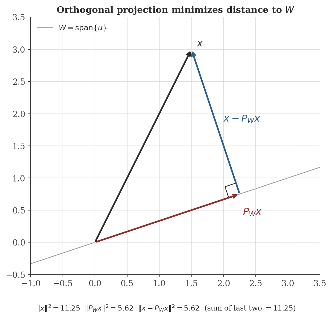
Given a subspace $W\subseteq V$ and $x\in V$, which point of $W$ is closest to $x$?

For $W=\operatorname{span}\{u\}$ one-dimensional, this reduces to the familiar $P_Wx = \dfrac{\langle x,u\rangle}{\langle u,u\rangle}u$ (no need for $u$ to be unit-length; the normalization is absorbed into the denominator).

8. Gram–Schmidt orthogonalization

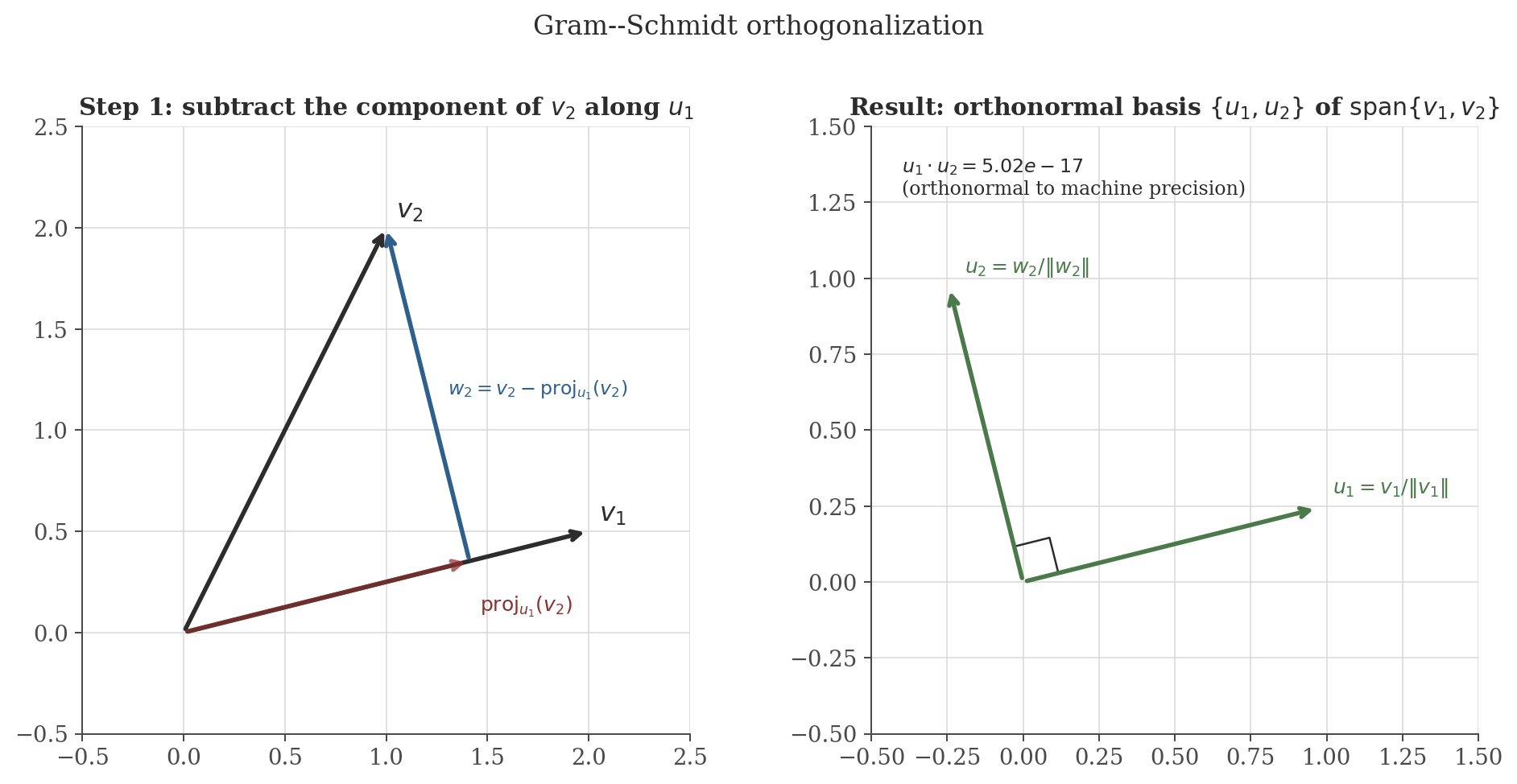
The best-approximation formula above needs an orthonormal basis of $W$ to start from. Gram–Schmidt builds one from an arbitrary basis $v_1,\ldots,v_k$ by inductively subtracting off the projection onto everything already orthogonalized:

Correctness is an induction on $j$ using exactly Section 7's theorem: assuming $w_1,\ldots,w_{j-1}$ (equivalently $u_1,\ldots,u_{j-1}$) are already an orthogonal basis of $W_{j-1}=\operatorname{span}\{v_1,\ldots,v_{j-1}\}$, the sum being subtracted is precisely $P_{W_{j-1}}v_j$, so $w_j = v_j - P_{W_{j-1}}v_j$ is (by the best-approximation theorem's proof) orthogonal to all of $W_{j-1}$, and nonzero because $v_j\notin W_{j-1}$ (linear independence of the original basis).

9. Computation

The figures above are generated by vector-spaces/generate_figures.py. The snippet below verifies the rank–nullity theorem on a concrete linear map, and confirms Cauchy–Schwarz including its equality case.

import numpy as np

# Rank-nullity on a concrete linear map R^4 -> R^3
A = np.array([
    [1.0, 2.0, -1.0, 0.0],
    [2.0, 4.0,  0.0, 1.0],
    [1.0, 2.0,  1.0, 1.0],
])
rank = np.linalg.matrix_rank(A)
n = A.shape[1]
nullity = n - rank
print(f"rank(A) = {rank}, nullity(A) = {nullity}, rank + nullity = {rank + nullity} (= n = {n})")

# Cauchy-Schwarz: strict for generic vectors, equality exactly when parallel
rng = np.random.default_rng(0)
x = rng.normal(size=5)
y = rng.normal(size=5)
print(f"generic:  |<x,y>| = {abs(x @ y):.4f}  <=  ||x|| ||y|| = {np.linalg.norm(x)*np.linalg.norm(y):.4f}")

y_parallel = 3.0 * x
lhs = abs(x @ y_parallel)
rhs = np.linalg.norm(x) * np.linalg.norm(y_parallel)
print(f"parallel: |<x,y>| = {lhs:.4f}  ==  ||x|| ||y|| = {rhs:.4f}")

Actual output:

rank(A) = 2, nullity(A) = 2, rank + nullity = 4 (= n = 4)
generic:  |<x,y>| = 1.0838  <=  ||x|| ||y|| = 1.8912
parallel: |<x,y>| = 2.2240  ==  ||x|| ||y|| = 2.2240

Confirms the rank–nullity theorem numerically (this particular $A$ has two independent columns, so a $2$-dimensional kernel), and Cauchy–Schwarz both as a strict inequality for generic vectors and as an exact equality once $y$ is forced parallel to $x$ — exactly the equality condition proved in Section 6.

10. Common pitfalls

11. Connections

• Matrices and eigenvalues. Column space, nullspace, rank, and eigenspaces are all subspaces in the sense of Section 2; the rank–nullity theorem proved here is what those notes' solvability and diagonalization arguments both quietly rely on.
• Regression (OLS). The fitted values $X\hat\beta$ in ordinary least squares are, by construction, the point of $\operatorname{col}(X)$ closest to $y$ in Euclidean norm — literally $P_{\operatorname{col}(X)}y$ in the notation of Section 7. The normal equations $X^\top(y-X\hat\beta)=0$ are exactly the orthogonality condition "$y-X\hat\beta \perp \operatorname{col}(X)$" from the best-approximation theorem, applied with $\langle\cdot,\cdot\rangle$ the standard dot product — OLS is orthogonal projection, not a separate idea that happens to look similar.
• Time series analysis. The partial autocorrelation function there is defined via "the best linear predictor of $X_t$ from $X_{t-1},\ldots,X_{t-h}$" — precisely $P_Wx$ of this note, with $W=\operatorname{span}\{X_{t-1},\ldots,X_{t-h}\}$ inside the (infinite-dimensional, but still inner-product) space of finite-variance random variables under $\langle Y,Z\rangle=\operatorname{Cov}(Y,Z)$.

12. References

• Axler, S. (2024). Linear Algebra Done Right (4th ed.). Springer.
• Halmos, P. R. (1974). Finite-Dimensional Vector Spaces (2nd ed.). Springer.
• Strang, G. (2016). Introduction to Linear Algebra (5th ed.). Wellesley-Cambridge Press.