Causal Inference

1. Potential outcomes and the fundamental problem

The Average Treatment Effect is $\mathrm{ATE}=E[Y_i(1)-Y_i(0)]$; the Average Treatment Effect on the Treated is $\mathrm{ATT}=E[Y_i(1)-Y_i(0)\mid D_i=1]$ — a different quantity in general, since the treated population need not resemble the population at large.

This framing matters because it makes precise what regression coefficients estimate under what conditions — and, by the same token, precisely why the regression methods note's OLS machinery does not automatically answer a causal question just because it is applied to observational data.

2. Identification assumptions, and why each is needed

• SUTVA (Stable Unit Treatment Value Assumption): unit $i$'s potential outcomes depend only on $i$'s own treatment, not on others' treatment status (no interference/spillovers) and there is only one version of "treated" (no hidden variation). Why needed: without it, $Y_i(1)$ is not even well-defined — "$i$ treated" could mean different things depending on who else is treated. Failure example: vaccinating one person in a population changes the disease exposure of untreated neighbors (herd immunity), so their $Y_i(0)$ is not a fixed number independent of the treatment assignment of others.
• Ignorability / unconfoundedness: $(Y_i(0),Y_i(1)) \perp D_i \mid X_i$ — conditional on observed covariates $X_i$, treatment assignment carries no information about potential outcomes. Why needed: without it, any comparison between treated and untreated groups conflates the treatment effect with pre-existing differences (Section 3 makes this precise). Failure example: sicker patients are more likely to receive an aggressive treatment, so treated and untreated patients differ in prognosis even before treatment, for reasons related to the very outcome being measured.
• Overlap / positivity: $0<P(D_i=1\mid X_i)<1$ for every value of $X_i$ with positive probability. Why needed: if some covariate stratum is always (or never) treated, there is no comparison group at that stratum to estimate a counterfactual from — the data simply contains no information about what would happen otherwise for those units, however large the sample.

3. What a naive comparison actually estimates

The selection bias term compares what the treated group's outcome would have been without treatment to the control group's actual outcome — a difference that has nothing to do with the treatment effect and vanishes only under ignorability, since $(Y_i(0))\perp D_i \Rightarrow E[Y_i(0)\mid D_i=1]=E[Y_i(0)\mid D_i=0]$. This decomposition is the formal version of "correlation is not causation": the naive comparison always estimates $\mathrm{ATT}+\text{selection bias}$, and every identification strategy in this note is a different way of arguing the selection bias term is zero (or of estimating it separately, as in DiD, Section 7).

4. Randomized experiments

This is immediate from Section 3: random assignment makes $D_i\perp(Y_i(0),Y_i(1))$ by construction (not by an assumption requiring justification from domain knowledge), so the selection bias term is exactly zero and $\mathrm{ATT}=\mathrm{ATE}$ (the treated group is, in expectation, a random sample of the whole population). This is precisely why randomized experiments are the benchmark the rest of this note's methods are built to approximate under weaker, observational conditions.

5. Instrumental variables and the Wald estimator

When treatment is not randomly assigned and no covariate set plausibly satisfies ignorability, an instrument $Z_i$ can substitute for randomization if it satisfies:

• Relevance: $\mathrm{Cov}(Z_i,D_i)\neq0$ — the instrument actually moves treatment.
• Exclusion restriction: $Z_i$ affects $Y_i$ only through $D_i$, not directly.
• Independence: $Z_i$ is as good as randomly assigned — independent of $(Y_i(0),Y_i(1))$.

Two-stage least squares generalizes this beyond a single binary instrument: regress $D$ on $Z$ (and covariates) to get fitted values $\hat D$, then regress $Y$ on $\hat D$. By the regression methods note's projection view of OLS (Section 2 there), $\hat D=P_{\mathrm{col}(Z)}D$ is exactly the part of $D$'s variation spanned by the instrument — 2SLS estimates the causal effect using only the treatment variation that the (assumed exogenous) instrument itself explains, discarding the rest as potentially confounded.

6. Regression discontinuity

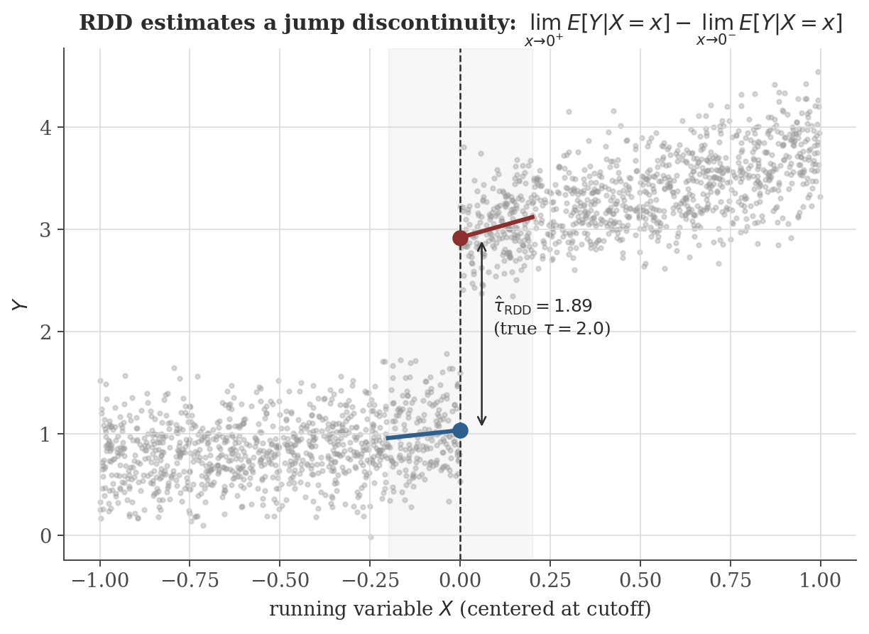
When treatment is assigned by whether a running variable $X_i$ crosses a known cutoff $c$ (e.g. a test score threshold for a scholarship), units just above and just below $c$ are, absent any special reason for anything else to also change discontinuously at $c$, comparable — differing systematically only in treatment status.

This is, precisely, a claim that $x\mapsto E[Y_i\mid X_i=x]$ has a jump discontinuity at $c$ in the sense of the continuity note (Section 4 there) — the one-sided limits both exist, and their difference (rather than their common value, which would signal no effect) is the causal estimate. In practice, each one-sided limit is estimated by local linear regression on data within a bandwidth $h$ of $c$, exactly the two separate fits shown in the figure below.

7. Difference-in-differences and parallel trends

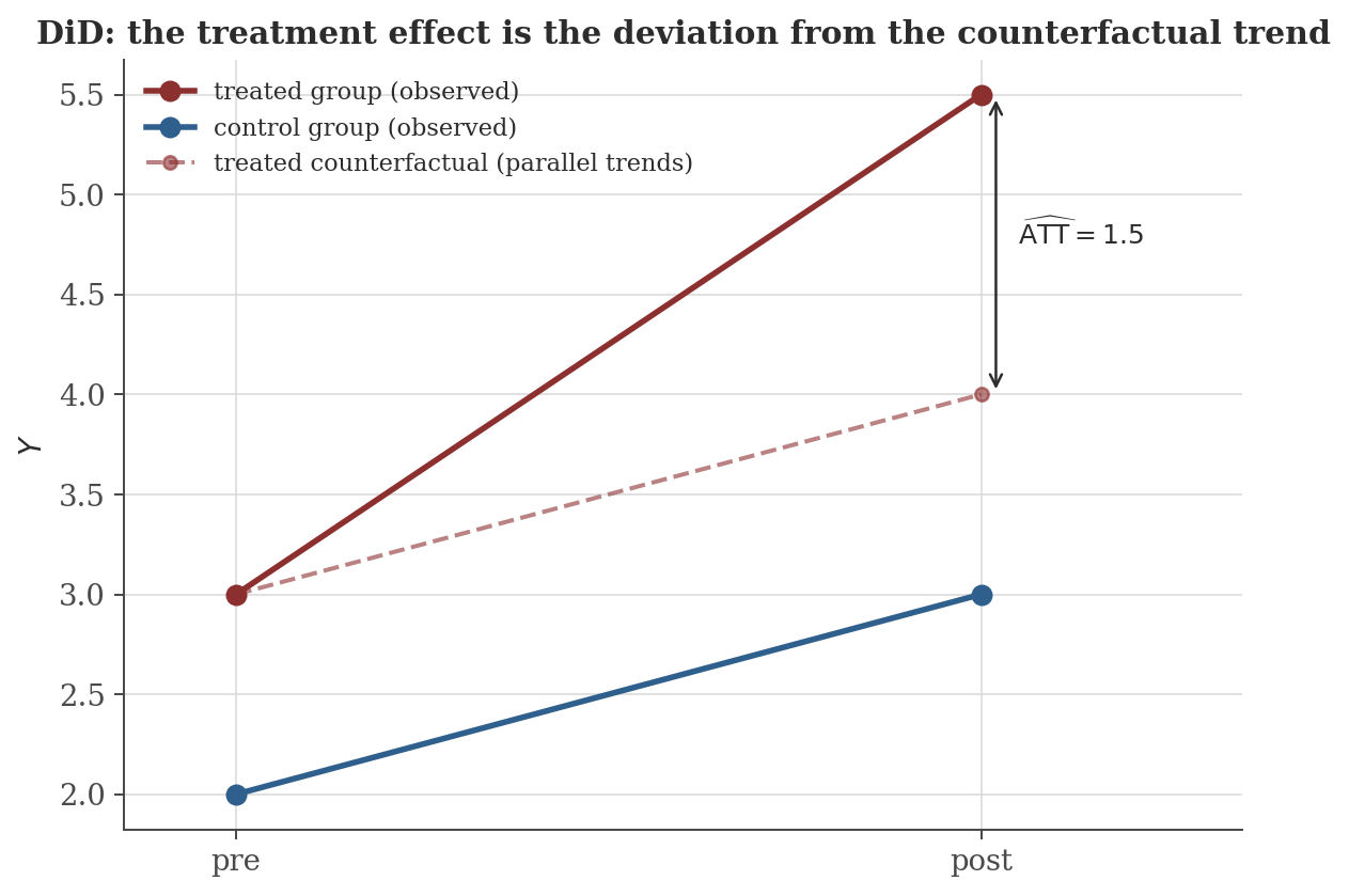
With outcomes observed pre- and post-treatment for both a treated and an untreated group, DiD identifies a treatment effect under an assumption weaker than unconditional ignorability:

8. The propensity score theorem

Conditioning on a high-dimensional $X_i$ to satisfy ignorability runs into overlap problems quickly (Section 2) — few or no comparable units may share an identical $X_i$. The propensity score, $e(X_i)=P(D_i=1\mid X_i)$, gives a way to condition on a single scalar instead.

This is a genuine dimension-reduction result, not merely a convenient approximation: it says that matching or weighting on the scalar $e(X_i)$ alone recovers exactly the same identification as conditioning on the full covariate vector $X_i$, provided the (unverifiable in general, but sometimes very plausible) ignorability assumption holds for $X_i$ in the first place. In practice $e(X_i)$ is unknown and estimated (typically by logistic regression of $D$ on $X$), which introduces its own estimation-error considerations not covered by the theorem itself.

9. Computation

The figures above are generated by causal-inference/generate_figures.py. The snippet below runs the RDD and DiD estimators shown in the figures, and separately verifies the omitted-variable-bias mechanism behind Section 3's selection-bias term: a naive regression that omits a confounder $X$ affecting both treatment and outcome is biased by exactly $\gamma\cdot\delta$, where $\gamma$ is $X$'s effect on $Y$ and $\delta$ is the regression coefficient of $X$ on $D$.

import numpy as np

rng = np.random.default_rng(2)
n = 5000
X = rng.normal(0, 1, n)                     # confounder
D = 0.5 * X + rng.normal(0, 1, n)           # treatment depends on the confounder
tau_true, gamma = 2.0, 1.5                  # true effect, and X's effect on Y
Y = 1 + tau_true * D + gamma * X + rng.normal(0, 1, n)

naive = np.linalg.lstsq(np.column_stack([np.ones(n), D]), Y, rcond=None)[0]
full = np.linalg.lstsq(np.column_stack([np.ones(n), D, X]), Y, rcond=None)[0]
delta = np.linalg.lstsq(np.column_stack([np.ones(n), D]), X, rcond=None)[0][1]

print(f"naive tau_hat (omits X): {naive[1]:.4f}   (true tau = {tau_true})")
print(f"full  tau_hat (controls X): {full[1]:.4f}")
print(f"predicted bias = gamma*delta = {gamma*delta:.4f}   actual bias = {naive[1]-tau_true:.4f}")

Actual output:

naive tau_hat (omits X): 2.5876   (true tau = 2.0)
full  tau_hat (controls X): 1.9987
predicted bias = gamma*delta = 0.5826   actual bias = 0.5876

The predicted and actual bias agree closely: controlling for the confounder recovers the true effect almost exactly, while omitting it produces bias numerically consistent with Section 3's decomposition — the naive coefficient is genuinely $\mathrm{ATE}+\text{selection bias}$, not merely "less accurate."

10. Common pitfalls

11. Connections

• Regression methods. Section 5's 2SLS is literally regression-methods.html's orthogonal-projection view of OLS applied twice; naive OLS of $Y$ on $D$ is exactly the Section 3 decomposition's biased comparison unless ignorability (or an equivalent design) holds.
• Continuity and limits. The sharp RDD estimand (Section 6) is precisely a one-sided-limit jump-discontinuity statement, and local linear regression is precisely how each one-sided limit is estimated in practice.
• Time series analysis. DiD's parallel-trends assumption implicitly requires understanding the untreated group's own trend as a legitimate forecast of the counterfactual — the same forecasting logic developed there, now applied as an identifying assumption rather than a prediction goal.

12. References

• Imbens, G. W., & Rubin, D. B. (2015). Causal Inference for Statistics, Social, and Biomedical Sciences. Cambridge University Press.
• Angrist, J. D., & Pischke, J.-S. (2009). Mostly Harmless Econometrics. Princeton University Press.
• Rosenbaum, P. R., & Rubin, D. B. (1983). The central role of the propensity score in observational studies for causal effects. Biometrika, 70(1), 41–55.
• Morgan, S. L., & Winship, C. (2014). Counterfactuals and Causal Inference (2nd ed.). Cambridge University Press.